Buildings-to-Grid Integration

Importance of Buildings-to-Grid Integration

By 2050, 70% of the world’s population is projected to live and work in cities, with buildings as major constituents. Buildings’ energy consumption contributes to more than 70% of electricity use. Future cities with innovative building operations have the potential to play a pivotal role in reducing energy consumption, curbing greenhouse gas emissions, while maintaining stable electric-grid operations. Buildings are physically connected to the electric power grid, thus it would be natural to understand the explicit coupling of decisions and operations of the two.

In this project, we present a mathematical framework for Buildings-to-Grid (BtG) integration in smart cities. The framework explicitly couples power grid and buildings’ control actions and operational decisions. This work analytically establishes that the BtG integration yields a reduced total system cost in comparison with decoupled designs where grid and building operators determine their controls separately or via other demand response schedules.

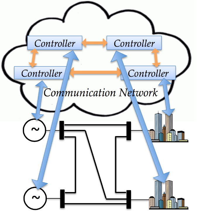
The below figure shows how local control actions of individual generators or distributed energy resources in power grids can communicate with local decisions of buildings. This yields a guaranteed energy savings, and most importantly, a more stable power grid operation in terms of voltage stability and frequency regulation.

The Computational Framework

Building dynamics are written in terms of the internal temperature of zones, external disturbances (such as ambient temperature and internal heat sources), and the control input which is essentially the HVAC power consumption. These dynamics can be written as:

$\begin{eqnarray*} \dot{T}_{\mathrm{wall}} & =& \dfrac{T_{\mathrm{amb}} -T_{\mathrm{wall}} }{CR_2}+\dfrac{T_{\mathrm{zone}} -T_{\mathrm{wall}} }{CR_1}+\frac{\dot{Q}_{\mathrm{sol}} }{C} \label{equ:buildingDynamics} \\ \dot{T}_{\mathrm{zone}} & = & \dfrac{T_{\mathrm{wall}} -T_{\mathrm{zone}} }{C_{\mathrm{zone}}R_1}+\dfrac{T_{\mathrm{amb}} -T_{\mathrm{zone}} }{C_{\mathrm{zone}}R_{\mathrm{win}}} +\frac{\dot{Q}_{\mathrm{int}} + \dot{Q}_{\mathrm{HVAC}} }{C_{\mathrm{zone}}}, \nonumber \end{eqnarray*}$

or more succinctly as an uncertain dynamic system:

(1) $\begin{equation*}~\begin{equation*}~\dot{\m x}_b(t) = \m A_b \m x_b(t) + \m B_{ u_{b}} \m u_b(t) + \m B_{w_{b}} \m w_b(t)\,,\,\, \end{equation*}$

where $x_b$ collects the two states (wall and zone temperatures), $u_b$ is the control input $\dot{Q}_{\mathrm{HVAC}}$ , and $w_b$ collects all disturbances. Note that tcooling load can be calculated as $\dot{Q}_{\mathrm{HVAC}}(t)=\mu_{\mathrm{HVAC}}P_{\mathrm{HVAC}}(t),$ where $P_{\mathrm{HVAC}}$ is the power consumed by the HVAC system, and $\mu_{\mathrm{HVAC}}$ is the coefficient of performance of the HVAC system.

The interesting part is that the control input of each building is explicitly expressed in the so-called swing equation of power networks, which models the dynamic energy transfer between buses and transmission lines. The swing equation for the $k$ th bus ( $k \in \mathcal{B}$ ) can be written asThe swing equation for the $k$ th bus ( $k \in \mathcal{B}$ ) can be written as

(2) $\begin{eqnarray*} M_k\ddot{\delta}_k(t)+D_k\dot{\delta}_k(t)&=&P_{k}(t)-P_{L_k}(t) -\displaystyle \sum_{j \in \mathcal{N}_k} b_{kj} \sin(\delta_k(t)-\delta_j (t)).~ \end{eqnarray*}$

The load at bus $k$ , $P_{L_k}(t)$ is described by

(3) $\begin{equation*}P_{L_k}(t)= P_{\mathrm{BL}_k}(t) + P_{\mathrm{bldg}_k}(t).\end{equation*}$

In (3), the first term $P_{\mathrm{BL}_k}(t)$ denotes the frequency-insensitive uncontrollable base load at bus $k$ , which is typically available via forecasts. The term $P_{\mathrm{bldg}_k}$ defines the load from buildings attached to bus $k$ participating in regulation. The building load is further decomposed as

$P_{\mathrm{bldg}} (t)=P_{\mathrm{HVAC}}(t)+P_{\mathrm{misc}}(t).$

The quantity $P_{\mathrm{HVAC}}(t)$ denotes the portion of controllable power consumption of buildings, while
$P_{\mathrm{misc}}(t)$ represents the uncontrollable miscellaneous power consumption such as lighting, computers, equipment, elevators—amounting to a building’s base-load. The coupling between buildings’ and power grids’ real time control actions can be seen through the $P_{\mathrm{HVAC}}(t)$ which appears in both, the building dynamics and the swing equation.

The computational framework we developed exploits this coupling to obtain localized control actions for generators (and OPF setpoints) in addition to 5-minute, HVAC setpoints for individual buildings. The below figures show the grid’s frequency (in Hz), the power generation, the zone temperatures (in Celsius) and HVAC setpoints for all buildings for MATPOWER’s case57 with 1822 commercial buildings and 7 generators for a 24-hour simulation.

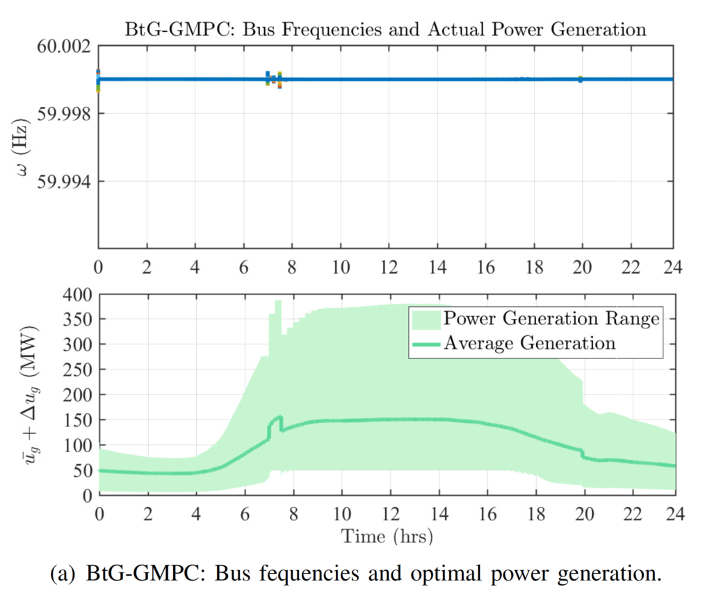
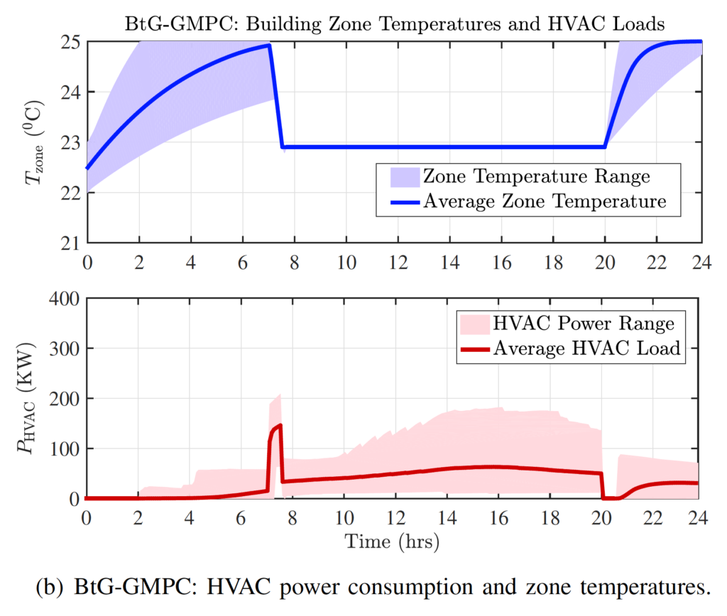
The figures and the numerical tests show that the proposed BtG integration algorithm maintains the grid’s stability, while reducing energy consumption. For more information, check the preprint of this work and this Github link for the codes.